The non-linear bicycle model considers longitudinal (x), lateral
(y), and yaw ![]() motion under the assumption of negligible
lateral weight shift, roll and compliance steer while traveling on
a smooth road. Our design of control strategy is to control both
longitudinal and lateral motions during hard braking and steering
maneuvers. Angular velocities of front and rear tires are added to
the states in order to investigate directional interactions
between longitudinal and lateral tire forces. In addition to these
five states, longitudinal and lateral positions and yaw angle with
respect to the fixed inertial coordinates are added to the dynamic
equation in order to refresh the vehicle position and orientation
in the simulation scene. Thus, the bicycle model used in our
simulator has 5 Degrees Of Freedom with 8 state equations.
The bicycle model developement presented here is based on
reference [1]. Figure 1 shows side and top
views of the vehicle using this bicycle model. Using free body
diagram shown in top view of Figure 1, the equations of motion are derived.
motion under the assumption of negligible
lateral weight shift, roll and compliance steer while traveling on
a smooth road. Our design of control strategy is to control both
longitudinal and lateral motions during hard braking and steering
maneuvers. Angular velocities of front and rear tires are added to
the states in order to investigate directional interactions
between longitudinal and lateral tire forces. In addition to these
five states, longitudinal and lateral positions and yaw angle with
respect to the fixed inertial coordinates are added to the dynamic
equation in order to refresh the vehicle position and orientation
in the simulation scene. Thus, the bicycle model used in our
simulator has 5 Degrees Of Freedom with 8 state equations.
The bicycle model developement presented here is based on
reference [1]. Figure 1 shows side and top
views of the vehicle using this bicycle model. Using free body
diagram shown in top view of Figure 1, the equations of motion are derived.
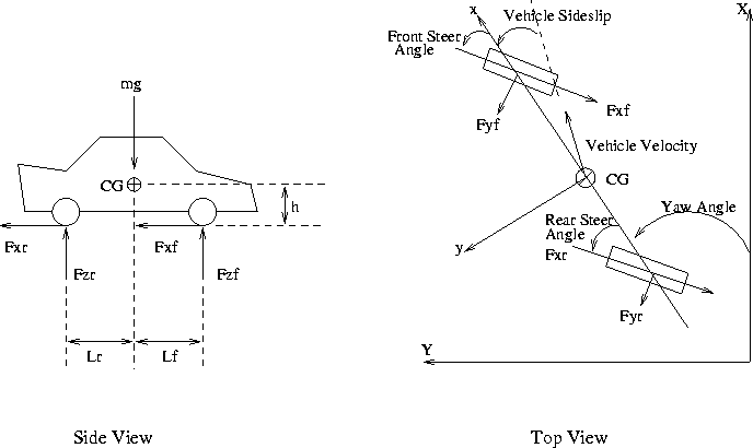
Figure 1: Free Body
Diagram of a Vehicle
Summing the longitudinal forces along the body x axis leads to
Where m is the mass of a vehicle, ![]() and
and ![]() are the
longitudinal and lateral components of the vehicle velocity
resolved along the body axis, r is the yaw rate, and
are the
longitudinal and lateral components of the vehicle velocity
resolved along the body axis, r is the yaw rate, and ![]() and
and ![]() are the front and rear wheel steering angles.
Summing the lateral forces along the body y axis gives
are the front and rear wheel steering angles.
Summing the lateral forces along the body y axis gives
The sum of the yaw moments about the car CG yields
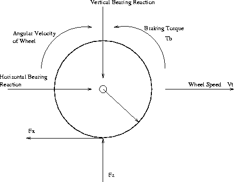
Figure 2: Free Body
Diagram of a Wheel
For the front and rear wheels, the sum of the torque about the axle, as shown in Figure 2, results in
![]()
Where, ![]() and
and ![]() are the angular velocities of the
front and rear wheels,
are the angular velocities of the
front and rear wheels, ![]() is the inertia of the wheel about the
axle,
is the inertia of the wheel about the
axle, ![]() is the wheel radius,
is the wheel radius, ![]() and
and ![]() are the
applied braking torques, and
are the
applied braking torques, and ![]() and
and ![]() are the applied
throttling torques for the front and rear wheels. All the vehicle
specifications are based on the 1984 Honda Accord [2]
with reasonable braking torques for front and rear tires. Yaw
angle is directly found by integrating the yaw rate. Since yaw
angle is with respect to the fixed coordinates, longitudinal and
lateral position with respect to the inertial fixed coordinates
are also found as follows.
are the applied
throttling torques for the front and rear wheels. All the vehicle
specifications are based on the 1984 Honda Accord [2]
with reasonable braking torques for front and rear tires. Yaw
angle is directly found by integrating the yaw rate. Since yaw
angle is with respect to the fixed coordinates, longitudinal and
lateral position with respect to the inertial fixed coordinates
are also found as follows.
![]()
![]()
Where, ![]() and
and ![]() denote the velocity components with respect
to the fixed inertial coordinates. Simple integration based on the
forth-order Runge-Kutta method is used to integrate the above eight
states in the simulation loop.
denote the velocity components with respect
to the fixed inertial coordinates. Simple integration based on the
forth-order Runge-Kutta method is used to integrate the above eight
states in the simulation loop.
The longitudinal and lateral forces from front and rear tires are
derived from the non-linear tire model discussed earlier. The
input variables for the tire model are front and rear normal loads
(
![]() and
and
![]() ), slip angles (
), slip angles (
![]() and
and
![]() ), and longitudinal slip ratios (
), and longitudinal slip ratios (
![]() and
and
![]() ). The normal forces of front and rear tires are
determined according to the instantaneous longitudinal
acceleration. Summing the moments about the rear contact patch
using the side view of Figure 1, normal load of front
tire is found as
). The normal forces of front and rear tires are
determined according to the instantaneous longitudinal
acceleration. Summing the moments about the rear contact patch
using the side view of Figure 1, normal load of front
tire is found as
![]()
Summing the moments about the front contact patch,
![]()
Where
![]() is the instantaneous longitudinal acceleration and h
is the height of the car CG from the ground.
is the instantaneous longitudinal acceleration and h
is the height of the car CG from the ground.
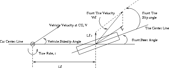
Figure 3: Slip Angle
of Front Wheel
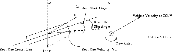
Figure 4: Slip Angle
of Rear Wheel
From Figure 3 and Figure 4, velocities of front and rear tires are determined by summing the velocity at CG and the velocities effected by the yaw rate. Thus, the slip angles of front and rear tires are found as
Also, the speed of the front and rear tires are calculated by the following equations.
![]()
![]()
Where,
![]() and
and
![]() represent the magnitude of the front
and rear tire axle velocities. To calculate the longitudinal slip, longitudinal
component of the tire velocity should be derived. The front and
rear longitudinal velocity components are found by
represent the magnitude of the front
and rear tire axle velocities. To calculate the longitudinal slip, longitudinal
component of the tire velocity should be derived. The front and
rear longitudinal velocity components are found by
![]()
![]()
Then, the longitudinal slip is determined according to the equation in tire model. Under braking conditions, longitudinal slip of front and rear tires are calculated by
![]()
![]()
Using the normal load, slip angle, longitudinal slip, and
non-linear tire model realistic longitudinal and lateral forces
are generated for the 5 DOF bicycle model.
References