![]()
![]()
Numerous applications such as air-traffic handling,
missile interception, anti-submarine warfare require the use of
discrete-time data to predict the kinematics of a dynamic object.
The use of passive sonobuoys which have limited power capacity
constrain us to implement target-trackers which are
computationally inexpensive. With these considerations in mind, we
analyze an
![]() -
-
![]() -
-
![]() filter to study its ability
to predict the object kinematics in the presence of noisy
discrete-time data.
filter to study its ability
to predict the object kinematics in the presence of noisy
discrete-time data.
There exists a significant body of literature which
addresses the problem of track-while-scan systems
[12], [5], [2] and
[1]. Sklansky [12] in his seminal paper
analyzed the behavior of an
![]() -
-
![]() filter. His analysis
of the range of values of the smoothing parameters
filter. His analysis
of the range of values of the smoothing parameters
![]() and
and
![]() which resulted in a stable filter constrained the
parameters to lie within a stability triangle. He also derived
closed form equations to relate the smoothing parameters for
critically damped transient response and the ability of the filter
to smooth white noise using a figure of demerit which was referred
to as the noise ratio. Finally he proposed, via a numerical
example, a procedure to optimally select the
which resulted in a stable filter constrained the
parameters to lie within a stability triangle. He also derived
closed form equations to relate the smoothing parameters for
critically damped transient response and the ability of the filter
to smooth white noise using a figure of demerit which was referred
to as the noise ratio. Finally he proposed, via a numerical
example, a procedure to optimally select the
![]() -
-
![]() parameters to minimize a performance index which is a function of
the noise-ratio and the tracking error for a specific maneuver.
Following his work, Benedict and Bordner [2] used
calculus of variations to solve for an optimal filter which
minimizes a cost function which is a weighted function of the
noise smoothing and the transient (maneuver following) response.
They show that the optimal filter is coincident with an
parameters to minimize a performance index which is a function of
the noise-ratio and the tracking error for a specific maneuver.
Following his work, Benedict and Bordner [2] used
calculus of variations to solve for an optimal filter which
minimizes a cost function which is a weighted function of the
noise smoothing and the transient (maneuver following) response.
They show that the optimal filter is coincident with an
![]() -
-
![]() filter with the constraint that
filter with the constraint that
![]() .
.
Numerous researchers using assumptions of the noise characteristics develop optimal filters [8], [10] and [3] which are commonly called Kalman Filters. Those filters were first introduced in the 60's by Kalman [6] and [7].
Kalata [4] proposed a new parameter
which he referred to as the tracking index to
characterize the behavior of
![]() -
-
![]() and
and
![]() -
-
![]() -
-
![]() filters. The tracking index was
defined as the ratio of the position maneuverability
uncertainty to the position measurement uncertainty.
He also presented a technique to vary the
filters. The tracking index was
defined as the ratio of the position maneuverability
uncertainty to the position measurement uncertainty.
He also presented a technique to vary the
![]() -
-
![]() -
-
![]() parameters as a function of the tracking index.
parameters as a function of the tracking index.
In this chapter, a detailed analysis of the
![]() -
-
![]() -
-
![]() filter is carried out. Section 2 discusses the bounds on the
smoothing parameters for a stable filter. This is followed by a
closed form derivation of the noise ratio for the
filter is carried out. Section 2 discusses the bounds on the
smoothing parameters for a stable filter. This is followed by a
closed form derivation of the noise ratio for the
![]() -
-
![]() -
-
![]() filter in Section 3. In Section 4, a
closed form expression for the steady state errors and a metric to
gauge the transient response of the filter are derived followed by
the optimization of the smoothing parameters for various cost
functions in Section 5. The chapter concludes with some remarks in
Section 6.
filter in Section 3. In Section 4, a
closed form expression for the steady state errors and a metric to
gauge the transient response of the filter are derived followed by
the optimization of the smoothing parameters for various cost
functions in Section 5. The chapter concludes with some remarks in
Section 6.
The
![]() -
-
![]() tracker is an one-step ahead
position predictor that uses the current error called the
innovation to predict the next position. The innovation is
weighted by the smoothing parameter
tracker is an one-step ahead
position predictor that uses the current error called the
innovation to predict the next position. The innovation is
weighted by the smoothing parameter
![]() and
and
![]() . These
parameters influence the behavior of the system in terms of
stability and ability to track the target. Therefore, it is
important to analyze the system using control theoretic aspects to
gauge stability and performance.
. These
parameters influence the behavior of the system in terms of
stability and ability to track the target. Therefore, it is
important to analyze the system using control theoretic aspects to
gauge stability and performance.
The form of the equations for the
![]() -
-
![]() tracker can be
derived by considering
the motion of a point mass with constant acceleration which is
described by integrating Newtons First Law yielding
tracker can be
derived by considering
the motion of a point mass with constant acceleration which is
described by integrating Newtons First Law yielding
![]() , where v is velocity and a is
acceleration. If the acceleration is negligible and the equation of
motion is written in discrete time where the initial condition
, where v is velocity and a is
acceleration. If the acceleration is negligible and the equation of
motion is written in discrete time where the initial condition
![]() and
and
![]() are substituted by the smoothed condition, the one-step ahead
prediction equation for an -
are substituted by the smoothed condition, the one-step ahead
prediction equation for an -
![]() tracker is obtained :
tracker is obtained :
The use of the equation of motion without neglecting the acceleration
would lead to the -
![]() tracker discussed later on, in this
work. Equation (1) states that between each time step, a
linear motion is assumed and the smoothed conditions
tracker discussed later on, in this
work. Equation (1) states that between each time step, a
linear motion is assumed and the smoothed conditions
![]() and
and
![]() are the initial conditions for each time step. The
smoothed conditions are derived using the innovation and the previous
states according to Equations (2) and
(3).
are the initial conditions for each time step. The
smoothed conditions are derived using the innovation and the previous
states according to Equations (2) and
(3).
The innovation in eq:ab_smooth_x and
(3) defined as
![]() represents the error between the observed and predicted
position. As can be seen,
represents the error between the observed and predicted
position. As can be seen,
![]() and , the smoothing parameter,
change the dynamics of the system. The input-output relationship
between the observed and predicted position,
and , the smoothing parameter,
change the dynamics of the system. The input-output relationship
between the observed and predicted position,
![]() ,
is referred to as the system in this work.
,
is referred to as the system in this work.
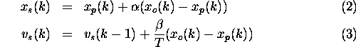
Since the prediction equation, eq:ab_predic, is in recursive form, it needs to be initialized. The initialization procedure requires two observed target positions to calculate the smoothed initial velocity. Therefore, the target position prediction begins with the third time step. The initial predicted target position is defined to be equal to the observed position at the second time step
leading to a zero initial innovation, which means that the smoothing parameter have no influence of the initial prediction. The smoothed initial velocity is calculated by the finite difference of the two observed target positions divided by the appropriate time,
According to eq:ab_smooth_x the smoothed position at the second time step equals the predicted target position at the same time. The first predicted position can therefore be calculated by the following equation:
![]()
which is an extrapolation of the first two observed target positions. Figure 1 illustrates the track initialization. It can be seen that the third predicted position is on the straight line formed by the first two observations and the first and the third position are equidistant from the second.
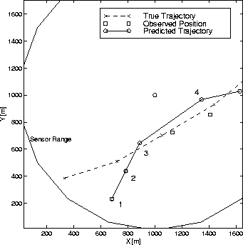
Figure 1: Target Track Initialization
The behavior of the system can be expressed in terms of the
smoothing parameters
![]() and ; furthermore, regions of stability
and different transient response characteristics can be specified in the -
and ; furthermore, regions of stability
and different transient response characteristics can be specified in the -
![]() space. Writing eq:ab_predic, (2) and
(3) in the z-domain and substituting
space. Writing eq:ab_predic, (2) and
(3) in the z-domain and substituting
![]() and
and
![]() into the prediction Equation (1) yields the
transfer function of the system in the z-domain G(z) as
follows,
into the prediction Equation (1) yields the
transfer function of the system in the z-domain G(z) as
follows,
which can now be used to determine the region of stability
of the -
![]() filter. Stability requires that the roots of the
characteristic polynomial lie within the unit circle in the
z-domain. The characteristic polynomial is given by the denominator of
eq:G_zdomain. To prove that the roots lie
within the unit circle, one can transform eq:G_zdomain
into the w-domain, mapping the unit circle of the z-domain to the
left half plane of the w-domain and applying one of the known
stability criteria in continuous domain. Another approach is to check
the stability directly in the z-domain using Jury's Stability
Test.
filter. Stability requires that the roots of the
characteristic polynomial lie within the unit circle in the
z-domain. The characteristic polynomial is given by the denominator of
eq:G_zdomain. To prove that the roots lie
within the unit circle, one can transform eq:G_zdomain
into the w-domain, mapping the unit circle of the z-domain to the
left half plane of the w-domain and applying one of the known
stability criteria in continuous domain. Another approach is to check
the stability directly in the z-domain using Jury's Stability
Test.
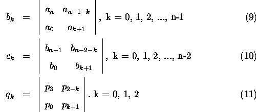
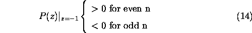
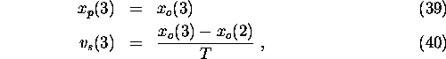
The Jury's Stability Test can be used to analyze the stability of the system without explicitly solving for the poles of the system. Therefore, it is used to determine the bounds on the parameters which result in a stable transfer function in the z-domain.
For a system with a characteristic equation P(z) = 0, where
![]()
and
![]() ;SPMgt; 0, we construct the table where the first row consists of the
elements of the polynomial P(z) in ascending order and the second row consists of
the parameters in descending order [9]. The table is
shown in Table 1.
;SPMgt; 0, we construct the table where the first row consists of the
elements of the polynomial P(z) in ascending order and the second row consists of
the parameters in descending order [9]. The table is
shown in Table 1.
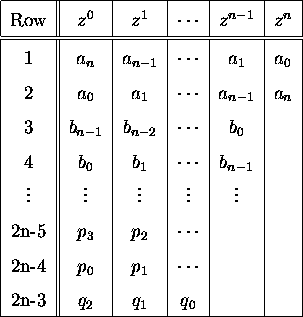
Table 1: General Form of Jury's Stability Table
where
Note, that the last row of the table contains only three elements. The Jury's test states that a system is stable if all of the following conditions are satisfied:
![]()
![]()
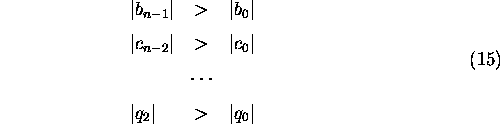
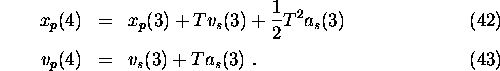
Exploiting this scheme for the characteristic polynomial of the
![]() -
-
![]() filter leads to the following Jury's table shown in Table 2.
filter leads to the following Jury's table shown in Table 2.
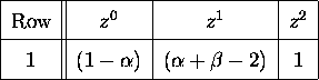
Table 2: Jury's Stability Table of the
![]() -
-
![]() Filter
Filter
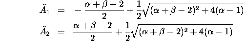
The condition that
![]() ;SPMgt; 0 is satisfied since
;SPMgt; 0 is satisfied since
![]() = 1. To
satisfy the constraint
= 1. To
satisfy the constraint
![]()
we require
![]()
which is equivalent to
To satisfy the constraint
![]()
we require
![]()
which can be rewritten as
To satisfy the constraint
![]()
we require
![]()
which can be rewritten as
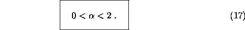
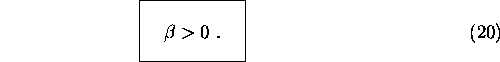
Equations 18, 21 and 24 defines the region
where
![]() and
and
![]() may lie for the tracker to be
stable. Plotting the boundaries of these constraints, one arrives at the
stability triangle shown in Figure (2).
may lie for the tracker to be
stable. Plotting the boundaries of these constraints, one arrives at the
stability triangle shown in Figure (2).
The stability area can be divided by the critical damped curve into an over-, and underdamped area as well as into areas with certain eigenfrequencies of the system. The system is said to be critically damped if the poles are coincident. Therefore, critical damping is obtained by solving the following equation.
since,
Solving eq:cdamp leads to the following relationship
for critical damped response of the filter.
The dashed line in Figure 2 corresponds to the solution
![]() and the dash-dot line to the solution
and the dash-dot line to the solution
![]() . eq:critdamp is
valid for all
. eq:critdamp is
valid for all
![]() , and the system is oscillating if
the poles in eq:z_roots contain a non-zero imaginary part. This can be seen
by using the transformation between z- and s-domain.
, and the system is oscillating if
the poles in eq:z_roots contain a non-zero imaginary part. This can be seen
by using the transformation between z- and s-domain.
We now show that, even though the smoothing parameters are chosen to be in the overdamped area, the system can oscillate under certain circumstances. These circumstances need to be investigated to achieve a specific transient response. Furthermore, expressions for the eigenfrequencies of the system will be derived.
The first part involves analyzing the space where
![]() is less than one
followed by the analysis for the region where we consider
is less than one
followed by the analysis for the region where we consider
![]() greater than one.
All areas discussed are also shown in
Figure 2. eq:z_roots shows that
if the system is underdamped, the z-poles become a complex conjugate
pair. In this case, eq:z_roots can be rewritten as follows:
greater than one.
All areas discussed are also shown in
Figure 2. eq:z_roots shows that
if the system is underdamped, the z-poles become a complex conjugate
pair. In this case, eq:z_roots can be rewritten as follows:
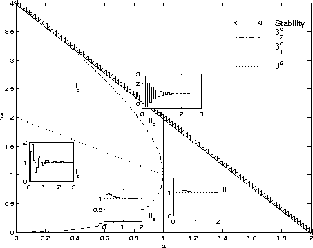
Figure 2: Regions of the - Tracker
Comparing eq:z2s with eq:z_roots2
yields the following equation for the eigenfrequency
![]() .
.
Equating
![]() to zero, which corresponds to the critically damped case,
simplifies Equation 30, resulting in Equation
27.
The effect of
to zero, which corresponds to the critically damped case,
simplifies Equation 30, resulting in Equation
27.
The effect of
![]() and
and
![]() on the eigenfrequency can be easily interpreted
using Equation 30 unlike Equation 26.
Representing the poles of
eq:z2s as a vector in the complex domain, as shown in
Figure 3, various regions of the
on the eigenfrequency can be easily interpreted
using Equation 30 unlike Equation 26.
Representing the poles of
eq:z2s as a vector in the complex domain, as shown in
Figure 3, various regions of the
![]() -
-
![]() space can be easily
analyzed.
space can be easily
analyzed.
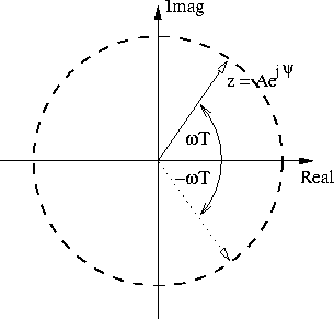
Figure 3: The Poles as a Vector in the Complex Domain
The highest frequency is obtained if the vector in Figure 3
lies on the real axis
and points to negative infinity, so that
![]() implying
implying
![]() which in
turn is on the critical damped curve corresponding to
which in
turn is on the critical damped curve corresponding to
![]() .
eq:omega can be used to determine when the real part of the poles changes
sign, which corresponds the vector in Figure 3 subtending an
angle
.
eq:omega can be used to determine when the real part of the poles changes
sign, which corresponds the vector in Figure 3 subtending an
angle
![]() to the real axis which corresponds to a frequency of
to the real axis which corresponds to a frequency of
![]() . If the denominator of the argument in eq:omega
becomes zero, the real part is also zero, and leads to the line
. If the denominator of the argument in eq:omega
becomes zero, the real part is also zero, and leads to the line
![]() illustrated by the dotted line in Figure 2.
This divides the region for
illustrated by the dotted line in Figure 2.
This divides the region for
![]() less than one into an area
where the poles have
positive and negative real parts as follows:
less than one into an area
where the poles have
positive and negative real parts as follows:
Although the regions
![]() and
and
![]() correspond to
the overdamped area as shown in Figure 2, the region
correspond to
the overdamped area as shown in Figure 2, the region
![]() corresponds to oscillatory dynamics with a
constant frequency of
corresponds to oscillatory dynamics with a
constant frequency of
![]() . Remembering that the vector in Figure 3
corresponding to the critical
damped curve
. Remembering that the vector in Figure 3
corresponding to the critical
damped curve
![]() lies on the real axes with a phase of
lies on the real axes with a phase of
![]() ,
any set of
,
any set of
![]() and
and
![]() in the region
in the region
![]() does not change the
phase since it only changes the magnitude of the vector.
Within the region
does not change the
phase since it only changes the magnitude of the vector.
Within the region
![]() the frequency of eq:omega
becomes complex which if substituted in eq:z2s, leads to a
negative real pole. For example, for the stability boundary
we have,
the frequency of eq:omega
becomes complex which if substituted in eq:z2s, leads to a
negative real pole. For example, for the stability boundary
we have,
![]()
which results in
![]()
The roots of the filter can now be represented as
![]()
which corresponds to an oscillatory response with a frequency of
![]() which cannot be derived from Equation 26.
which cannot be derived from Equation 26.
If
![]() becomes greater than 1, the roots of
eq:z_roots are never negative, so the
above approach cannot be applied. When
becomes greater than 1, the roots of
eq:z_roots are never negative, so the
above approach cannot be applied. When
![]() , Equation 26
leads to the following two poles.
, Equation 26
leads to the following two poles.
where
As can be seen in eq:z_roots3, in the region
![]() , one pole is oscillating with
, one pole is oscillating with
![]() and the
other corresponds to an overdamped mode with zero frequency.
and the
other corresponds to an overdamped mode with zero frequency.
The
![]() -
-
![]() tracker is obtained by neglecting the
acceleration term in the equation of motion of a point mass. Deriving a
tracker which includes the acceleration, is a better representation of the
equation of motion, leading to the
tracker is obtained by neglecting the
acceleration term in the equation of motion of a point mass. Deriving a
tracker which includes the acceleration, is a better representation of the
equation of motion, leading to the
![]() -
-
![]() -
-
![]() tracker.
tracker.
The equation of the higher order one-step ahead prediction
is the same as for the
![]() -
-
![]() tracker with an additional
term representing the influence of the acceleration.
tracker with an additional
term representing the influence of the acceleration.
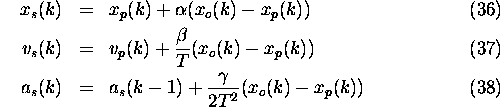
The additional information about the acceleration allows us to predict the velocity of the target as well. eq:abg_predic_v.
where the smoothed kinematic variables are again calculated by weighting the innovation as follows:
Similar to the
![]() -
-
![]() filter are the assumptions about the
initial conditions of the
filter are the assumptions about the
initial conditions of the
![]() -
-
![]() -
-
![]() filter. Since the
velocity is also predicted, eq:abg_predic_v, the initialization
requires three observed target positions. Equations 4
and 5 are now used one time step ahead:
filter. Since the
velocity is also predicted, eq:abg_predic_v, the initialization
requires three observed target positions. Equations 4
and 5 are now used one time step ahead:
and the smoothed initial acceleration is calculated by the finite differnece of the two initial velocities as follows:
![]()
The first target position prediction is now available at the fourth time step:
Depending on the target, the initial acceleration might be neglected
and set to be zero. Thus, the amount of required initial observed points
reduces to the requirements of an
![]() -
-
![]() filter.
filter.
Applying the Laplace Transform to eq:abg_predic_x to
(39) and solving for the ratio
![]() leads to the transfer function in z-domain which is
leads to the transfer function in z-domain which is
Equation 45 can now be used to determine the bounds of
![]() ,
,
![]() and
and
![]() for stability.
For this complex system, the Jury's
Stability Test is used as described in Section 2.2, to determine the
region of stability.
for stability.
For this complex system, the Jury's
Stability Test is used as described in Section 2.2, to determine the
region of stability.
Writing the coefficients of the characteristic polynomial in
Jury's Table, and calculating the determinants
![]() ,
,
![]() and
and
![]() (Equation 9) yield the Table 3.
(Equation 9) yield the Table 3.
Table 3: Jury's Stability Table of the
![]() -
-
![]() -
-
![]() Filter
Filter
The condition
![]() is satisfied since
is satisfied since
![]() . To satisfy the
constraint
. To satisfy the
constraint
![]() , the coefficients require
, the coefficients require
![]() ,
which is equivalent to
,
which is equivalent to
Substituting z=1 and applying the constraint
![]() ,
requires satisfaction of the inequality
,
requires satisfaction of the inequality
![]()
which can be rewritten as
Satisfying the constraint
![]() , for odd n, yields
, for odd n, yields
which is the same constraint for
![]() and
and
![]() as for the
as for the
![]() -
-
![]() tracker. The final condition
tracker. The final condition
![]() requires
requires
Observing eq:abg_constraint and knowing the fact that
![]() is always negative within the stability area,
we have:
is always negative within the stability area,
we have:
![]()
This statement leads to the constraint on
![]() for which the
for which the
![]() -
-
![]() -
-
![]() tracker is stable, which is
tracker is stable, which is
Figure 4 illustrates the bounding surfaces which include
the stable volume in the
![]() -
-
![]() -
-
![]() space based on
eq:alpha1, (48), (49) and
(52).
space based on
eq:alpha1, (48), (49) and
(52).
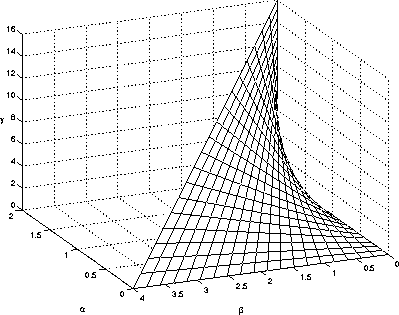
Figure 4: Stability Area of the
![]() -
-
![]() -
-
![]() Tracker
Tracker
It is desirous to divide the stability volume into regions
which are characterized by specific class of transient responses
such as, underdamped, overdamped, and critically damped. However,
the difficulty of factorizing the characteristic polynomial of the
transfer function in the
![]() -
-
![]() -
-
![]() space prompt
us to conceive of a new space which we refer to as the
a-b-c space. In this space, the characteristic polynomial is represented as
space prompt
us to conceive of a new space which we refer to as the
a-b-c space. In this space, the characteristic polynomial is represented as
where the second order factor has a form which is identical to the
characteristic equation of the
![]() -
-
![]() filter and the
third pole is real and is located at z=-c.
Comparing the denominator of
eq:abg_Gz with eq:abc_poly the following transformation is
derived:
filter and the
third pole is real and is located at z=-c.
Comparing the denominator of
eq:abg_Gz with eq:abc_poly the following transformation is
derived:
The usefulness of this transformation, becomes evident when
one derives the stability volume of the
![]() -
-
![]() -
-
![]() filter. Since, c is constrained to lie within -1 and 1, and
the a-b space resembles the
filter. Since, c is constrained to lie within -1 and 1, and
the a-b space resembles the
![]() -
-
![]() space, the stability
volume in the a-b-c space is a prism (Figure 5)
with a triangular cross-section
which is derived from the
space, the stability
volume in the a-b-c space is a prism (Figure 5)
with a triangular cross-section
which is derived from the
![]() -
-
![]() filter. Mapping the stability
prism in the a-b-c space to the
filter. Mapping the stability
prism in the a-b-c space to the
![]() -
-
![]() -
-
![]() space using
Equation (54), we rederive the stability volume
illustrated in Figure (4).
space using
Equation (54), we rederive the stability volume
illustrated in Figure (4).
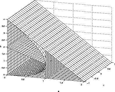
Figure 5: Stability Prism in the a-b-c Space
Since, the pair of poles of eq:abc_poly which are
functions of a and b are responsible for oscillation of the system,
the a-b-c space is divided by extruding the lines which divide the
stability triangle of the
![]() -
-
![]() filter (Figure 2),
in the c dimension.
These surfaces, shown in Figure 5, are transformed using
eq:abg_trans to the
filter (Figure 2),
in the c dimension.
These surfaces, shown in Figure 5, are transformed using
eq:abg_trans to the
![]() -
-
![]() -
-
![]() space. Figure 6 shows the surfaces in the
space. Figure 6 shows the surfaces in the
![]() -
-
![]() -
-
![]() space corresponding to each
critically damped surface of the a-b-c space.
Figure 7 shows the transformation of the two surfaces
dividing the stability area at a=1 and b=2-a.
space corresponding to each
critically damped surface of the a-b-c space.
Figure 7 shows the transformation of the two surfaces
dividing the stability area at a=1 and b=2-a.
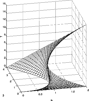
Figure 6: Critical Damped Surfaces of the
![]() -
-
![]() -
-
![]() Space
Space

Figure 7: Mapping between a-b-c Space and
![]() -
-
![]() -
-
![]() Space
Space
Observing Figures (6) and (7), illustrates the
fact that for
![]() , the third order tracker reduces to the
, the third order tracker reduces to the
![]() -
-
![]() tracker. Substituting
tracker. Substituting
![]() in the transfer function
(eq:G_zdomain), results in a pole zero cancellation at z=1, resulting
in a second order tracker. From eq:abg_trans, we can infer that
c equals -1 when
in the transfer function
(eq:G_zdomain), results in a pole zero cancellation at z=1, resulting
in a second order tracker. From eq:abg_trans, we can infer that
c equals -1 when
![]() , and furthermore a and
b degenerate to
, and furthermore a and
b degenerate to
![]() and
and
![]() . The cross-section at c=-1 therefore corresponds
to the
. The cross-section at c=-1 therefore corresponds
to the
![]() -
-
![]() tracker. Note that c=0 does not result in degenerating the
tracker. Note that c=0 does not result in degenerating the
![]() to the
to the
![]() -
-
![]() filter.
filter.References