The fuzzy logic theory overcomes the difficulty of defining an explicit relationship between the current system states and the actions required to achieve a certain system performance by using linguistic rules. These rules could be determined with an experts knowledge or simply by stating the required cause effect relation in common language, which has the form of if-then statements. Furthermore, the rules could be learned during some kind of training algorithm [4].
This chapter uses a simple fuzzy controller to introduce
the fuzzy elements interactions before exploring a more
sophisticated representation of the fuzzy algorithm. The rule base
of the proposed fuzzy filter is determined by an analogy to the
optimal solution of the rest-to-rest maneuver of a second order
system [3], where we propose a relationship between
the damping and stiffness determined by the rest-to-rest maneuver
to the smoothing parameter ![]() and
and ![]() .
.
The interaction between the fuzzy elements is first shown on an single-input-single-output example, followed by description of a general fuzzy logic algorithm. Suppose one is interested in keeping a constant flow out of a valve, one would open the valve if the flow slows down and vice versa. The appropriate rules may formulated as:
| | | | |
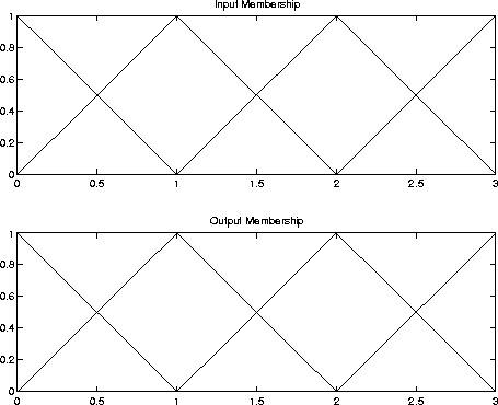
Figure 1: Input and Output Membership function of the Example
For reasons of generality and brevity it is convenient to
introduce a label for each rule. Since each input could possible
be related to every output, a matrix of rules with the size of
[number of input membership functions ![]() number of output
membership functions] is constructed. Thus, the four given example
rules are labeled as shown above. The first rule,
number of output
membership functions] is constructed. Thus, the four given example
rules are labeled as shown above. The first rule, ![]() , for
instance, shows that the first input membership function is
combined with the fourth output membership function. This labeling
scheme is also convenient with the use of confidences of each
rule. A confidence of a rule expresses the belief in this rule,
and is a gain between zero and one. If more than one rule is
applied to one input membership function, the confidences should
be normalized such that the sum equals one. This is not
necessarily required, but its use permits scaling the output. The
general form of the fuzzy rule can now be written as:
, for
instance, shows that the first input membership function is
combined with the fourth output membership function. This labeling
scheme is also convenient with the use of confidences of each
rule. A confidence of a rule expresses the belief in this rule,
and is a gain between zero and one. If more than one rule is
applied to one input membership function, the confidences should
be normalized such that the sum equals one. This is not
necessarily required, but its use permits scaling the output. The
general form of the fuzzy rule can now be written as:
where ![]() and
and ![]() are the input
and output variables of dimension m and n. Each input and
output set contains
are the input
and output variables of dimension m and n. Each input and
output set contains ![]() and
and ![]() membership functions. For a
single input-single output fuzzy system the rule and confidence
matrixes are of size [
membership functions. For a
single input-single output fuzzy system the rule and confidence
matrixes are of size [ ![]() ], whereas for
multi-input-output fuzzy systems the rule and confidence
matrixes are of size [
], whereas for
multi-input-output fuzzy systems the rule and confidence
matrixes are of size [ ![]() ] thus avoiding higher order matrixes.
] thus avoiding higher order matrixes.
Since the input and often the output are crisp values,
processing the crisp values using linguistic rule bases requires the input to be
fuzzyfied and the output to be defuzzyfied. This procedure
assigns a certain numerical value refered to as degrees of membership
functions ( ![]() ) and vice versa for degrees on output
memberships (
) and vice versa for degrees on output
memberships ( ![]() ) a crisp output value. Since both schemes differ from
each other, they are discussed separately. The input fuzzyfication
assigns degrees of active membership functions to a crisp value. As
shown as in Figure 2, Part A the example input, x, has non-zero
membership in the input set zero and small with the degree of
) a crisp output value. Since both schemes differ from
each other, they are discussed separately. The input fuzzyfication
assigns degrees of active membership functions to a crisp value. As
shown as in Figure 2, Part A the example input, x, has non-zero
membership in the input set zero and small with the degree of
![]() and
and ![]() . To explain the output
defuzzyfication we need to construct first the fuzzy output according
to the fuzzy inference. Since this example input activates the
membership functions of zero (i=1) and small (i=2), which means
that all rules
. To explain the output
defuzzyfication we need to construct first the fuzzy output according
to the fuzzy inference. Since this example input activates the
membership functions of zero (i=1) and small (i=2), which means
that all rules ![]() and
and ![]() , where
, where ![]() , need to be
evaluated. According to the example rules there are two rules
, need to be
evaluated. According to the example rules there are two rules ![]() and
and
![]() . The first rule suggests: If the input is zero then the output
should be large, which means that the output membership function large
is activated. Since the input has a fractional membership of the input
set zero, the corresponding membership of the output set large needs also be
adjusted. For purpose of demonstration the simple truncation algorithm
is applied, where the output set large is truncated to the membership
of the input set
. The first rule suggests: If the input is zero then the output
should be large, which means that the output membership function large
is activated. Since the input has a fractional membership of the input
set zero, the corresponding membership of the output set large needs also be
adjusted. For purpose of demonstration the simple truncation algorithm
is applied, where the output set large is truncated to the membership
of the input set ![]() . Similarly the second fuzzy
influence can be constructed. Part C in Figure 2 visualizes this
algorithm. Note, that a multivariable
input space is mapped in a hyper membership set, where the inputs are
combined with respect to each rule. Furthermore, since rule
. Similarly the second fuzzy
influence can be constructed. Part C in Figure 2 visualizes this
algorithm. Note, that a multivariable
input space is mapped in a hyper membership set, where the inputs are
combined with respect to each rule. Furthermore, since rule ![]() and rule
and rule ![]() are firing, a compromise between these two
suggested outputs needs to be achieved. During this step, the
and operation is carried out which is either the algebraic (Addition) or
logic (Maximum) operator. Combining the two fuzzy influences with the addition
operator yields the fuzzy output shown in Figure 2, Part D. This
linguistic (fuzzy) output is quite certain that the output should be
somewhat medium and also somewhat large, let us say somewhat between
medium and large. The human operator might be able to interpret this
linguistic terms as opposed to most technical applications requiring a crisp
value. This final step of defuzzyfication loses all the important
information about the fuzzy output by reducing it to one crisp value,
the defuzzyfied output.
are firing, a compromise between these two
suggested outputs needs to be achieved. During this step, the
and operation is carried out which is either the algebraic (Addition) or
logic (Maximum) operator. Combining the two fuzzy influences with the addition
operator yields the fuzzy output shown in Figure 2, Part D. This
linguistic (fuzzy) output is quite certain that the output should be
somewhat medium and also somewhat large, let us say somewhat between
medium and large. The human operator might be able to interpret this
linguistic terms as opposed to most technical applications requiring a crisp
value. This final step of defuzzyfication loses all the important
information about the fuzzy output by reducing it to one crisp value,
the defuzzyfied output.
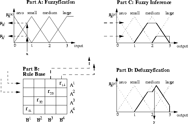
Figure 2: Fuzzy Example Algorithm
The above example of a fuzzy algorithm contains a lot of motivation for use of fuzzy systems instead of equations describing the same process. However, implementing the fuzzy algorithm in a lot more complex requiring a more sophisticated process. Figure 3 recalls the steps taken by the fuzzy decision process.
The fuzzyfication maps the crisp value ![]() into the
fuzzy set
into the
fuzzy set ![]() . A common approach is the singleton
fuzzyfication where a binary membership is used. eq:single
represents the singleton method.
. A common approach is the singleton
fuzzyfication where a binary membership is used. eq:single
represents the singleton method.
The fuzzy influence combines the input sets with the output
sets based on the fuzzy rules, which results in the fuzzy set with
the membership ![]() for each rule and the fuzzy
rule base
for each rule and the fuzzy
rule base ![]() combining the separate
rules. The individual membership functions are calculated as:
combining the separate
rules. The individual membership functions are calculated as:
![]()
where ![]() is the AND-operator. If
is the AND-operator. If ![]() is multivariate,
each input set needs to be related to the other according to:
is multivariate,
each input set needs to be related to the other according to:
![]()
Combining the individual sets with the OR-operator ( ![]() )
yields the input-output-relation:
)
yields the input-output-relation:
where the indices i and j are within the range 1 to ![]() and 1 to
and 1 to ![]() . The fuzzy intersection
AND may be a algebraic product operator or a the
logic minimum operator. Whereas, the OR intersection can be
derived using the addition or maximum operator. These are the most
popular fuzzy intersection, where the logic operators in the
literature referred to as Mamdani intersection. Table 1
summarizes the most popular fuzzy intersections.
. The fuzzy intersection
AND may be a algebraic product operator or a the
logic minimum operator. Whereas, the OR intersection can be
derived using the addition or maximum operator. These are the most
popular fuzzy intersection, where the logic operators in the
literature referred to as Mamdani intersection. Table 1
summarizes the most popular fuzzy intersections.
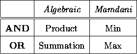
Table 1: Common Fuzzy Intersections
The fuzzy rule base eq:rulebase can now be used to
generate the fuzzy output distribution for a given input set
![]() obtained by the fuzzyfication process. This
procedure is known as the compositional rule of inference, which may
be written as:
obtained by the fuzzyfication process. This
procedure is known as the compositional rule of inference, which may
be written as:
![]()
where `` ![]() '' is the composition operator and
'' is the composition operator and ![]() is the degree of output membership functions. The composition
procedure is similar to the example in Figure 2 where the
suggested output by each rule is truncated and than added to get the
final output distribution. Therefore, the composition operator performs
a comparison of the two membership functions and summarizes over all
possible values of
is the degree of output membership functions. The composition
procedure is similar to the example in Figure 2 where the
suggested output by each rule is truncated and than added to get the
final output distribution. Therefore, the composition operator performs
a comparison of the two membership functions and summarizes over all
possible values of ![]() . The composition operator for fuzzy
sets defined on a continuous domain in a more general expression may be
written as:
. The composition operator for fuzzy
sets defined on a continuous domain in a more general expression may be
written as:
![]()
and similarly in the discrete domain as:
For a singleton fuzzyfication Equation 8 reduces to:
where ![]() is the discrete value closest to the input
is the discrete value closest to the input
![]() .
.
Figure 4 illustrates the rule base given in Equation 5 for the fuzzy example introduced above. The universe is discrete, and the AND and OR operators are represented with the algebraic operations.
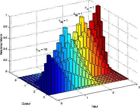
Figure 4: Relational Matrix of the above Example
The relational matrix represents the shape of the fuzzy input and
output sets and shows the underlying fuzzy algorithm. Observing the
relational matrix in Figure 4, illustrates the mapping of the
input space to the output space with respect to the four example rules
(four spikes). The influence of the rule confidences on the
relational matrix is also shown in Figure 4, where the
confidence of the rule ![]() is reduced to
is reduced to ![]() . Thus, the
weight of the output according to this rule reduces and the spike of
the relational matrix is therefore scaled down. If the input is
singleton fuzzyfied, eq:mubs can be applied, which means that
the fuzzy output is given by the appropriate column of the discrete
relational matrix. Figure 5 shows such a slice through the
relational matrix at the crisp input value of 1.25.
. Thus, the
weight of the output according to this rule reduces and the spike of
the relational matrix is therefore scaled down. If the input is
singleton fuzzyfied, eq:mubs can be applied, which means that
the fuzzy output is given by the appropriate column of the discrete
relational matrix. Figure 5 shows such a slice through the
relational matrix at the crisp input value of 1.25.
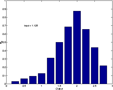
Figure 5: Discrete Fuzzy Output Membership
As mentioned before, the fuzzy, imprecise output,
![]() needs to be transformed to a crisp value using
a defuzzyfication scheme. The most popular defuzzyfication is the
center of gravity defuzzyfication, which is defined for the continuous
and discrete domain as follows:
needs to be transformed to a crisp value using
a defuzzyfication scheme. The most popular defuzzyfication is the
center of gravity defuzzyfication, which is defined for the continuous
and discrete domain as follows:
Exploiting the eq:cogd and applying algebraic operators, reduces the calculation of the output to [1]:
where ![]() are the weights similar to the joints of an Associative Memory Network
(AMN). The relationship between the confidences and the weights can be
shown to be:
are the weights similar to the joints of an Associative Memory Network
(AMN). The relationship between the confidences and the weights can be
shown to be:

where ![]() is the center of the
is the center of the ![]() output membership
function. For a singleton input fuzzyfication eq:cogd2 reduces
to:
output membership
function. For a singleton input fuzzyfication eq:cogd2 reduces
to:

This representation is less computational expensive as opposed to storing the relational matrix and carrying out the matrix operations.
Unlike the fixed gain ![]() -
- ![]() filter the fuzzy logic
based
filter the fuzzy logic
based ![]() -
- ![]() filter changes the smoothing parameter,
filter changes the smoothing parameter,
![]() and
and ![]() , as a function of the maneuver error and
error rate with the tracking performance comparable to a
Kalman filter, but without modeling a target system and a sensor
noise model. Furthermore, the computational cost is less
than that of the Kalman filter. Moreover, the fuzzy
algorithm reaches a decision by considering several different
situations at the same time resulting in a more human like
decision.
, as a function of the maneuver error and
error rate with the tracking performance comparable to a
Kalman filter, but without modeling a target system and a sensor
noise model. Furthermore, the computational cost is less
than that of the Kalman filter. Moreover, the fuzzy
algorithm reaches a decision by considering several different
situations at the same time resulting in a more human like
decision.
The maneuver error is now defined as the difference between
the observed position and the predicted position of the target. Since,
the filter estimates the targets future position, the maneuver error
at the current time influences the choise of the appropriate smoothing
parameter ![]() and
and ![]() . The maneuver error at the current time
may be written as:
. The maneuver error at the current time
may be written as:
Besides the information ``How close the prediction is to the true target position'', the change of the maneuver error is also an important fact since different action must be taken whether the maneuver error is about to increase or decrease. The error rate is defined as follows:
For purpose of generality of the target tracker, normalization of the maneuver error and error rate are desired. Chan [2] introduced an effective normalization scheme, where the normalization denominator is variable and depends on the magnitude of the error. The following three situations may occur:
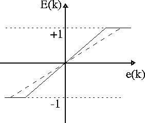
Figure 6: Error Normalization Scheme
Since the normalized maneuver error lies within the interval [-1,1], the maximum absolute maneuver error rate is 2. Similar to the above normalization scheme the error rate is also transformed into the interval [-1,1] according to the following equations:
This normalization scheme might be applied for each dimension
separately, where every normalized error and error rate contains the
information about the relative position of prediction and observation
(sign of the error). In a multivariable dimensional space one could
calculate the magnitude of the error and the error rate, and use those
to determine the appropriate ![]() and
and ![]() . This is proposed by
Chan [2] and the corresponding error magnitude are defined as:
. This is proposed by
Chan [2] and the corresponding error magnitude are defined as:

where the summations are carried out over the number of dimensions. These error and error rate magnitude lie within the interval [0,1]. On the contrary, the relative position of the prediction to the observation and the direction of changing the error are important to choose an appropriate control. Figure 7 illustrates the four situations.
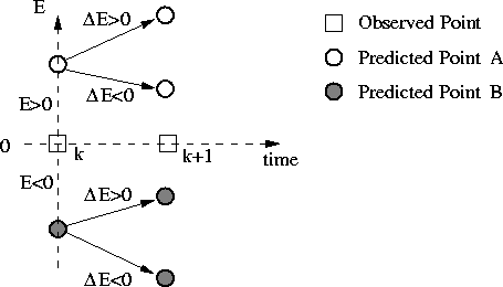
Figure 7: Development of Maneuver Error
The predicted position ``A'' in Figure 7 exhibits a positive maneuver error and a positive error rate increases the error of the next time step, whereas a negative error rate decreases the next error. On the other hand, a positive error rate for the predicted position ``B'' in Figure 7 decreases the maneuver error of the next time step. Likewise, a negative error rate induces the opposite effect.
Hence, a normalized representation of the error and error rate is given in Equations (16)-(18) and eq:ner, a general set of input membership functions can be defined. With regard to the normalization scheme, the input membership functions are generated as shown as in Figure 8. The fact that large errors are mirrored into the normalized bounds -1 and +1 leads to a larger region of support (ROS) of the negative-large (nl) and positive-large (pl) membership functions. Furthermore, the other membership functions shrink around zero together.
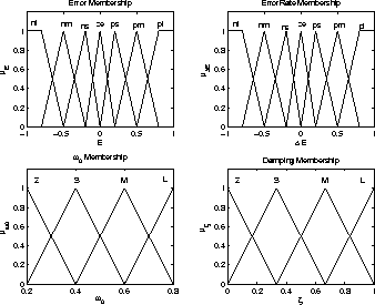
Figure 8: Membership Functions
The fuzzy logic rule base is built by combining the input
membership sets via the linguistic rules with the output
membership sets. The linguistic rules are of the form of eq:rules, where every possible input combination should be
covered. In case of the seven error and seven error rate input
sets shown in Figure 8, a minimum of 49 rules is required.
To increase the modeling capability a input combination of the
maneuver error and error rate may call different output membership
functions at the same time with the use of continuous confidences
[1]. Determining the rules is difficult and might be done
with the help of experts knowledge about the system [2].
In Chans work this expert's knowledge is used to determine the
specific amount of the smoothing parameter ![]() and
and ![]() .
The proposed fuzzy filter exploits an analogy from system
control theory, the rest-to-rest maneuver of a second order system
[3], to define appropriate rules.
.
The proposed fuzzy filter exploits an analogy from system
control theory, the rest-to-rest maneuver of a second order system
[3], to define appropriate rules.
The rest-to-rest maneuver requires a mass at rest to move as quickly as possible to another desired position of rest. The control law is modeled in the form of a non-linear spring-damper system shown in Figure 9. The coordinate system is fixed at the desired final position of rest, so that the first rest is expressed as an initial condition, and the controller of the rest-to-rest maneuver is designed to exhibit Lyupanov stability. The results of this work [3] are used to determine the 49 rules as explained in the following section.

Figure 9: Rest-to-Rest Maneuver
The transfer function of a spring-mass-dashpot system shown in Figure 9 can be represented in continuous time domain as:
where ![]() and
and ![]() are the undamped eigenfrequency and
the damping ratio. The transfer function of eq:r2rtf is
later used to define a relation between the smoothing parameter
are the undamped eigenfrequency and
the damping ratio. The transfer function of eq:r2rtf is
later used to define a relation between the smoothing parameter
![]() and
and ![]() , and the undamped eigenfrequency and the
damping ratio. The non-linear control law is defined in
[3] as follows:
, and the undamped eigenfrequency and the
damping ratio. The non-linear control law is defined in
[3] as follows:
![]()
where the constants ![]() are determined
to satisfy the above mentioned performance. The solution of the
original problem, the rest-to-rest maneuver, with an initial
position error and zero initial velocity is shown in
Figure 10.
are determined
to satisfy the above mentioned performance. The solution of the
original problem, the rest-to-rest maneuver, with an initial
position error and zero initial velocity is shown in
Figure 10.
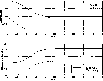
Figure 10: States and Control of the Rest-to-Rest Maneuver
We can infer from Figure 10 that the stiffness increases from
a non-zero value and the damping starts at zero. The closer the
mass to the final position, the higher the stiffness and damping.
This knowledge may now be used to determine the rules according to
which the control action is taken. A convinient structure of
writing these rules is shown in Table (2). Within
this table all possible input combinations are captured, since the
normalized error, Equations (16)-(18), is
entered in the first row and the normalized error rate, eq:ner, is entered in the first column. The original
rest-to-rest maneuver, explained above, is represented in
Table 2 at the row ![]() equals zero,
where large errors require small stiffness and
damping and zero error requires large stiffness and
damping. For similar reasons, the column with zero error
rate requires large stiffness and damping, trying to keep
the error and error rate small. As shown as in Figure 7
positive error and negative error rate exhibits the same situation
as negative error and positive error rate. Thus, the
Table 2 is mirrored symmetrical about the two
main-diagonals, which is emphasized by the light and dark gray
table entries. The gray table entries are determined by the use of
the modified rest-to-rest maneuver, where the initial rest
position is changed to different values of initial position and
velocity. For instance, the rule of positive medium
normalized error and positive medium normalized error rate
are obtained by setting the initial velocity and the initial
position to 0.5 as shown in Figure 11. The rule table
entry in the upper right and lower left rectangulars are obtained
with the same method.
equals zero,
where large errors require small stiffness and
damping and zero error requires large stiffness and
damping. For similar reasons, the column with zero error
rate requires large stiffness and damping, trying to keep
the error and error rate small. As shown as in Figure 7
positive error and negative error rate exhibits the same situation
as negative error and positive error rate. Thus, the
Table 2 is mirrored symmetrical about the two
main-diagonals, which is emphasized by the light and dark gray
table entries. The gray table entries are determined by the use of
the modified rest-to-rest maneuver, where the initial rest
position is changed to different values of initial position and
velocity. For instance, the rule of positive medium
normalized error and positive medium normalized error rate
are obtained by setting the initial velocity and the initial
position to 0.5 as shown in Figure 11. The rule table
entry in the upper right and lower left rectangulars are obtained
with the same method.
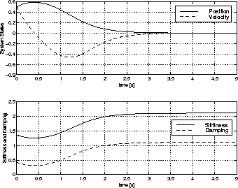
Figure 11: States and Control of the Rest-to-Rest Maneuver for non-zero
initial position and velocity
Underlying to this method is the following rule observed by Figure 7:
If the error decreases by itself (positive error and negative error rate and
vise versa), do not apply a large control (small stiffness and
damping), only if the error is small and the error rate is large
increase the damping of the system to prevent overshoot!|
If the error increases by itself, increase the damping moderate to
counteract this situation
| |
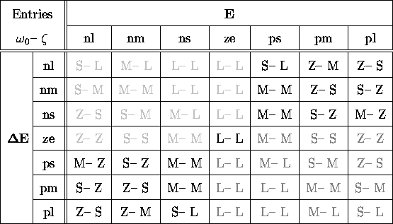
Table: Fuzzy Rule Base (Compare the linguistic Terms with Figure 8)
With the knowledge of the fuzzy rule base, Table 2, and the membership sets defined in Figure 8 the fuzzy relational matrix can now be derived according to eq:rulebase. Using the singleton input-fuzzyfication and the Center of Gravity Method to defuzzyfy the controllers output, the control surfaces shown in Figure 12 can be calculated.
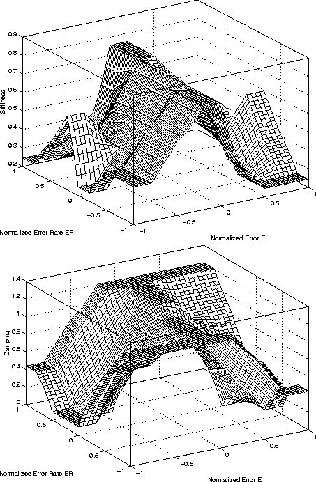
Figure 12: Stiffness and Damping Control Surface
Since the fuzzy controller is defined in terms of stiffness
and damping, it is required to express those terms as
smoothing parameter ![]() and
and ![]() . For this purpose we
recall the transfer function of the
. For this purpose we
recall the transfer function of the ![]() -
- ![]() filter
derived in Chapter
filter
derived in Chapter ![]() . The discrete transfer
function, eq:G_zdomain, shall be mapped into another
discrete domain where the terms stiffness and damping are defined.
Thus, the area of the unit circle of the z-domain is transformed
into the left half plane, often referred to as the w-domain. This
mapping is described by the following equation:
. The discrete transfer
function, eq:G_zdomain, shall be mapped into another
discrete domain where the terms stiffness and damping are defined.
Thus, the area of the unit circle of the z-domain is transformed
into the left half plane, often referred to as the w-domain. This
mapping is described by the following equation:
Applying this
transformation to the transfer function of eq:G_zdomain,
yields the transfer function of ![]() -
- ![]() filter with
respect to the w-domain.
filter with
respect to the w-domain.
The w-domain exhibits similar behavior
to the continuous s-domain since their stability regions are both
defined in the left half plane. This similarity is used to relate
the stiffness and damping to the smoothing parameter ![]() and
and
![]() . Comparing the characteristic polynomial of eq:r2rtf
with this of eq:G_wdomain leads to the following
relationship:
. Comparing the characteristic polynomial of eq:r2rtf
with this of eq:G_wdomain leads to the following
relationship:
Applying the transformation eq:albezo to the control
surface shown in Figure 12 yields finally to the
input-output-relationship between maneuver error and error rate
and the smoothing parameter ![]() and
and ![]() , which is shown
in Figure 13. During this mapping we assumed the direct
relationship between stiffness and eigenfrequency.
, which is shown
in Figure 13. During this mapping we assumed the direct
relationship between stiffness and eigenfrequency.
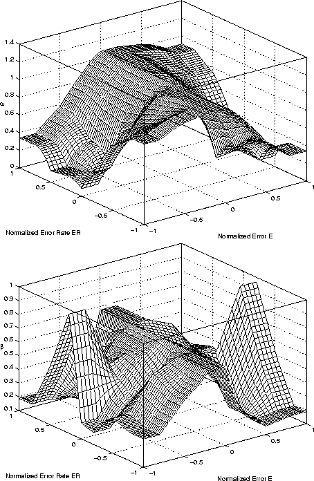
Figure 13: Smoothing Parameter ![]() and
and ![]() Control Surface
Control Surface
This chapter proposed a Fuzzy Logic Algorithm applied to the
standard ![]() -
- ![]() filter developed in
Chapter
filter developed in
Chapter ![]() . Unlike the fixed gain
. Unlike the fixed gain ![]() -
- ![]() filter, the fuzzy logic approach adapts the smoothing parameter
filter, the fuzzy logic approach adapts the smoothing parameter ![]() and
and
![]() as a function of the maneuver error and error rate. Thus,
the adaptive
as a function of the maneuver error and error rate. Thus,
the adaptive ![]() -
- ![]() filter is capable of tracking
various types of maneuvers whereas the fixed
filter is capable of tracking
various types of maneuvers whereas the fixed ![]() -
- ![]() filter can
only be optimized for one trajectory and certain sensor noise.
filter can
only be optimized for one trajectory and certain sensor noise.
The fuzzy logic algorithm is first illustrated via single-input-single-output
example and is discussed in detail in section 2.2
following the scheme illustrated in Figure 3. It is
shown how the fuzzy relational matrix can be created using the
input and output membership sets and the fuzzy rules. Finally, the relational
matrix is used to calculate the output fuzzy set ( ![]() ) which
is defuzzyfied for further usage.
) which
is defuzzyfied for further usage.
The final section discusses the implementation of the fuzzy logic algorithm into
the target tracking process. The linguistic rule base is
determined by an analogy to the rest-to-rest maneuver, where the
system variables, stiffness and damping, are
derived. A relationship between those system variables and the
smoothing parameters ![]() and
and ![]() is proposed to conclude
with the control surfaces shown in Figure 13.
is proposed to conclude
with the control surfaces shown in Figure 13.References